最新的 UIC 井级 VI 级于 2010 年设立,旨在规范 GS 的 CO 2注入,具有所有 UIC 井级中最严格的许可要求。UIC VI 类核心规定是划定审查区域 (AoR),即 GS 项目周围的区域,由于注入压力增加,该区域可能对 USDW 造成危害。AoR 边界基于地下流体流动和压力传播的高度复杂计算模型的预测,结合了原地和注入流体、注入地层和周围限制区域的物理和化学特性的详细描述。在 AoR 内,必须确定流体流出注入地层的潜在管道,并根据需要采取纠正措施,以防止注入流体和排开的孔隙水影响 USDW。而且,虽然目前只有一口积极注入 UIC VI 级油井,但仍有一百多个许可证正在接受技术审查,并且自《通货膨胀减少法案》通过以及扩大对 GS 的财政激励措施以来,这一数字迅速增长(图 2 ) 。
图 2 — 过去 2 年提交的 UIC VI 类申请数量
按州分组)。
资料来源:美国 EPA/B3 Insight
在 UIC VI 类之前的所有 UIC 井类中,UIC I 类危险废物注入井的许可与 UIC VI 类注入井的许可最相似,特别是在预先许可的场地特征要求方面。对于 UIC I 类危险废物注入,操作员必须证明废物在危险期间(目前定义为 10,000 年)将留在注入区域内。为此,需要识别、收集和汇总流体特性、岩石特性和操作活动(与 UIC VI 级许可的要求类似),以支持数千年来注入流体运动的建模。由于许多 UIC I 类危险废物注入井靠近 GS 感兴趣的区域(所有危险废物注入井的近四分之三位于德克萨斯州和路易斯安那州的墨西哥湾沿岸地区),毫无疑问,之前的一些评估可以和应用于 UIC VI 类场地特征描述。然而,由于遍布 19 个州的 UIC I 类注入井不足 1,000 个,其中只有约 15% 是 UIC I 类危险废物注入井,因此地理覆盖范围和高井密度区域都受到限制。
II 类潜望镜
另一方面,有超过 150,000 个 UIC II 类注入井用于注入与石油和天然气生产相关的流体,分布在包括阿拉斯加和夏威夷在内的 33 个州。UIC II 类注入井包括用于处理常规石油开采和地下天然气储存期间带到地面的流体的井(UIC II 类井的 22%)、用于注入流体以提高油气采收率的井(占 UIC II 类井的 76%)。 UIC II 类井),以及用于注入液态碳氢化合物用于地下储存的井(UIC II 类井的 2%)。图3显示了各州的井分布情况。四个州(德克萨斯州、加利福尼亚州、堪萨斯州和俄克拉荷马州)拥有超过 10,000 个 UIC II 类注入井,约占总库存的 75%。14 个州占 UIC II 类注水井总数的近 95%。
图3’II类注入井按州分布
。
资料来源:美国 EPA/B3 Insight
每口 UIC II 级注入井都提供了窥视黑暗地下的机会,为寻求地下可视性的 CCS 公司提供了线索。虽然许可证要求不像 UIC I 类危险废物注入井或 UIC VI 类注入井那么严格(特别是关于场地特征的范围和随后的长期现场监测),但 UIC II 类注入井的运营商或所有者必须定期测量和报告其油井的运行特征,包括月注入量、月平均井口压力和月最大井口压力。传统上,这些测量的目的是监测法规对允许的注入速率和压力限制的遵守情况,同时提供井性能的粗略评估。但是,当这个广泛的数据集提供了可以跨越数十年的操作记录,与其他注入井和地下特性相结合时,可以实现更大的价值——地质地层压力对流体注入的响应的高分辨率空间和时间特征广阔的地理区域。
Carbon Capture and Sequestration: The Pressures of Selecting the Perfect Site
Decades of experience injecting fluids into the ground has revealed a fundamental truth: No two injection sites are the same. A thorough understanding of site-specific conditions is essential to ensure safe and secure long-term subsurface disposal of carbon dioxide.
Source: inkoly/Getty Images
Geologic sequestration (GS) of carbon dioxide (i.e., the “S” in CCS [carbon capture and sequestration]) is an immediately available technology with considerable potential to reduce anthropogenic carbon dioxide emissions. But, to loosely quote Shakespeare, there’s a rub. Decades of experience injecting fluids into the ground has revealed a fundamental truth: No two injection sites are the same. Variability in fluid and rock properties (often across distances that can be measured by the throw of a stone), differences in injection well construction, and contrasting operational practices can lead to profound differences in how injected fluid moves through subsurface formations, how that fluid is retained in the rock pore space, and what inadvertent effects may result from injecting fluid into this pore space that is already occupied by groundwater. Every location, every project, and every well has idiosyncrasies. A thorough understanding of site-specific conditions is essential—from planning to construction to injection to site closure—in order to ensure safe and secure long-term subsurface disposal of carbon dioxide. Luckily, in many areas of GS interest, there is a data-rich source of subsurface and operational insight: Underground Injection Control (UIC) Class II wells.
This is Big In 2021, 2.7 billion tonnes carbon dioxide equivalent (CO2e) of greenhouse gases (GHGs) were released into the atmosphere from large direct-emitting facilities (i.e., facilities emitting more than 25,000 tonnes of CO2e per year) in the United States, approximately half of all US GHG atmospheric emissions. Seven states—Texas, Louisiana, Indiana, Pennsylvania, Florida, Ohio, and California—each emitted greater than 100 million tonnes of CO2e, accounting for 43% of the US’s large direct-emitting facilities total. Add Illinois and Alabama to the list, and these nine states accounted for 50% of total large facility emissions (Fig. 1).
Fig. 1—2021 CO2e emissions of GHG from large direct-emitting facilities (more than 25,000 tonnes of CO2e per year). MtCO2e = million tonnes of CO2 equivalent.
Source: US EPA
Texas, the biggest state GHG emitter, accounted for approximately one-sixth (466 million tonnes of CO2e) of the 2021 total from these large direct-emitting facilities. If the entirety of Texas GHG emissions (of which approximately 90% is carbon dioxide) were captured, injected, and stored as a supercritical fluid (i.e., a fluid at a temperature above its critical temperature (88°F for CO2) and at a pressure above its critical pressure (1,070 psi for CO2), with liquid-like density and gas-like viscosity, that would equate to roughly 5 billion bbl (or approximately 200 billion gal) sequestered underground. While that may seem like a staggeringly large number (and it is), consider that, in 2021, 9.3 billion bbl of water associated with oil and gas operations were injected in Texas. Taken as a whole, the current scale of yearly nationwide oil and gas water injection is roughly equivalent to the volume needed for permanent geologic storage of GHGs from large direct-emitting sources. From this volumetric perspective, GS is a meaningful and realistic tool for abatement of atmospheric carbon emissions.
A Class Act In the early 1980s, the US Environmental Protection Agency (EPA) established initial requirements for the Underground Injection Control (UIC) Program, promulgated under the Safe Drinking Water Act and the Resource Conservation and Recovery Act, to regulate underground injection of fluids. Since the program’s inception, six well classes have been established to manage injection of a variety of hazardous and nonhazardous wastes, with the purpose of protecting underground sources of drinking water (USDWs) and preventing adverse human health effects. Currently, there are more than 750,000 UIC wells nationwide.
The most recent UIC well class, Class VI, was established in 2010 to regulate CO2 injection for GS, with the most rigorous permitting requirements of all UIC well classes. A core UIC Class VI stipulation is delineation of an area of review (AoR), the region surrounding a GS project where potential exists for endangerment of USDWs because of increased pressure from injection. AoR boundaries are based on predictions from highly complex computational models of fluid flow and pressure propagation in the subsurface, incorporating detailed descriptions of physical and chemical properties of the in-place and injected fluids, the injection formation, and the surrounding confining zones. Within the AoR, potential conduits for fluid movement out of the injection formation must be identified and corrective action taken as needed to prevent both injected fluid and displaced pore water from affecting USDWs. And, while there currently is only one actively injecting UIC Class VI well, there are more than a hundred permits under technical review, with this number growing rapidly since passage of the Inflation Reduction Act and its expanded financial incentives for GS (Fig. 2).
Fig. 2—Number of submitted UIC Class VI applications, grouped by state, over the last 2 years.
Source: US EPA/B3 Insight
Of all the UIC well classes preceding UIC Class VI, the permitting of UIC Class I hazardous waste injection wells is most like that for UIC Class VI injection wells, particularly regarding pre-permitting site characterization requirements. For UIC Class I hazardous waste injection, operators must demonstrate that the waste will stay within the injection zone for as long as it remains hazardous (currently defined as a period of 10,000 years). To do so requires identification, collection, and aggregation of fluid properties, rock properties, and operational activity (as similarly required for UIC Class VI permitting) to support modeling of injected fluid movement over millennia. As many of these UIC Class I hazardous waste injection wells are close to areas of GS interest (nearly three-quarters of all hazardous waste injection wells are in the Gulf Coast region of Texas and Louisiana), undoubtedly, some of this previous assessment can and should be leveraged for UIC Class VI site characterization. However, because there are fewer than 1,000 UIC Class I injection wells throughout 19 states, only approximately 15% of which are UIC Class I hazardous waste injection wells, both geographic coverage and areas of high well density are limited.
Class II Periscopes On the other hand, there are more than 150,000 UIC Class II injection wells used to inject fluids associated with oil and gas production, located within 33 states including Alaska and Hawaii. UIC Class II injection wells include wells for disposal of fluids brought to the surface during conventional petroleum extraction and underground natural gas storage (22% of UIC Class II wells), wells used for injection of fluids for enhanced oil and gas recovery (76% of UIC Class II wells), and wells used for injection of liquid hydrocarbons for underground storage (2% of UIC Class II wells). Fig. 3 shows the distribution of wells by state. Four states (Texas, California, Kansas, and Oklahoma) have more than 10,000 UIC Class II injection wells, accounting for roughly 75% of the total inventory. Fourteen states account for nearly 95% of the total number of UIC Class II injection wells.
Fig. 3—Distribution of Class II injection wells by state.
Source: US EPA/B3 Insight
Each UIC Class II injection well provides an opportunity to peer into the murky subsurface, offering clues for CCS companies seeking subsurface visibility. While permit requirements are not as onerous as they are for UIC Class I hazardous waste injection wells or UIC Class VI injection wells (particularly regarding the extent of site characterization and subsequent long-term site monitoring), operators or owners of UIC Class II injection wells must regularly measure and report the operational characteristics of their wells, including monthly injected volume, monthly average wellhead pressure, and monthly maximum wellhead pressure. Conventionally, the purpose of these measurements is to monitor regulatory adherence to permitted injection rate and pressure limits while providing a cursory assessment of well performance. But far greater value can be realized when this expansive data set, providing an operational record that can span decades, is combined with other injection well and subsurface properties—a high-resolution spatial and temporal characterization of geologic formation pressure response to fluid injection over a broad geographic area.
But this is where it gets murky—again. Despite general consistency in reporting rules, how, where, and when this data gets reported varies widely between states. Additionally, data usability can range from excellent to challenging, depending on measurement and reporting quality. Therefore, rigorous and laborious collection, quality assurance and control, integration, and standardization processes are required to provide a clarifying view. Furthermore, translating measurements made at the wellhead to a description of subsurface conditions requires a painstaking effort to match well construction and completion history with well operation status while further conditioning the results with other measures of fluid, rock, and well properties.
But the effort pays an enormous dividend: a multidimensional view of the subsurface showing when, where, and how fluid injection affects the formation pressure, observed through aggregation of thousands of individual subsurface periscopes (Fig. 4). And the implications are significant. Know the past and present, and you have a much greater chance of reasonably describing the future.
Fig. 4—3D distribution of water injected in the Permian Basin during the past 5 years, shown at the point of subsurface injection. Symbol sizes represent cumulative injected volume, with injection into shallower formations shaded blue and deeper formations shaded red.
Source: B3 Insight
Truth Be Told There is much legitimacy to statistician George Box’s statement “All models are wrong, but some are useful.” But usefulness is undoubtedly tied to the availability, accessibility, and quality of data used to construct, constrain, and validate models. The better the input data, generally, the better the predictions—and, ultimately, the better ability to plan projects and avoid costly modifications and mistakes. To seed and verify the computational models used to predict pressure propagation and fluid movement, particularly for UIC Class VI AoR delineation, requires static (i.e., the rocks, the wells) and dynamic (i.e., the fluid injection rate, the pressure) characterization of the injection site. And, arguably, the most valuable measured data is that which captures the dynamic relationship between injection rate and pressure, particularly as the relationship can change over time. Individually, UIC Class II injection wells provide local understanding of well operation and injection formation conditions and how those conditions change over the life of the injection well. Collectively, these wells provide insight into ultimate disposal capacity for a formation by tracking the full trajectory of pressure change related to the historical volume of fluid injected.
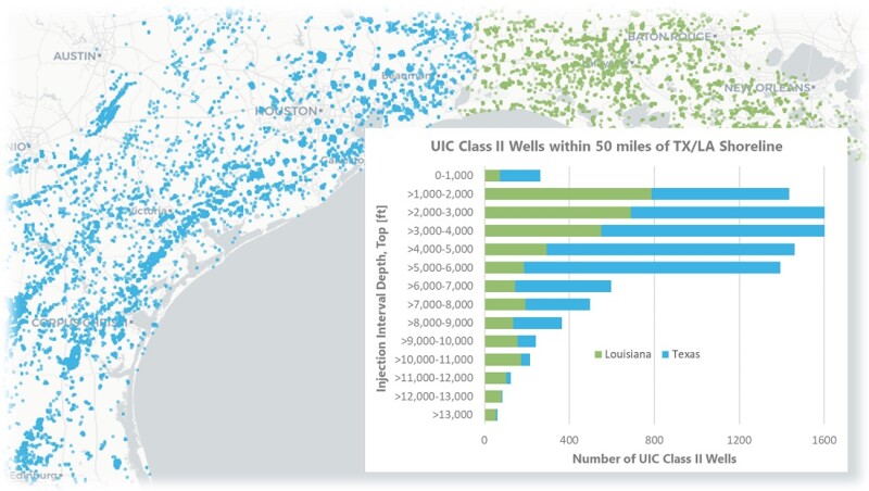
Fortunately, in numerous areas of GS interest, many of the 150,000 UIC Class II injection wells penetrate potential target formations considered for carbon injection, providing invaluable truth about formation pressure response to fluid injection. For example, large direct-emitting facilities within 50 miles of the shoreline in Texas and Louisiana account for more than 10% of the United States’ total, making this one of the more highly concentrated areas of point-source GHG emissions in the country (Fig. 5). And underneath lies thousands of feet of Miocene and Oligocene sedimentary rock potentially capable of sequestering vast amounts of CO2. Serendipitously, nearly 10,000 UIC Class II injection wells have been drilled in this area, with the majority constructed to inject into these Miocene and Oligocene formations. Both individually and in the aggregate, these wells provide a precious source of site-specific information about injection formation characteristics and the ability of these formations to accommodate large fluid volumes injected over decades. And, as GS moves from nascent to broad execution, with a permitting process that can take years and millions of dollars to complete, the more insight that can be immediately accessed and leveraged, the more economically, expeditiously, and responsibly will consequential (and essential) emissions abatement be achieved.
Fig. 5—Gulf Coast region UIC Class II wells. Texas well locations are shaded blue, and Louisiana well locations are shaded green. The inset chart shows the distribution of wells within 50 miles of the shoreline relative to the top depth of the injection interval.