The Ultimate Showdown in Eagle Ford Production Forecasting
This article presents a comparative study evaluating four machine-learning approaches, including three deep-learning methods, for forecasting gas and condensate production over a 5-year horizon.
Source: Igor Borisenko/Getty Images
Machine learning provides a valuable data-driven alternative to traditional methods for production forecasting in complex unconventional assets such as the Eagle Ford Shale. This article presents a comparative study evaluating four machine-learning approaches, including three deep-learning methods, for forecasting gas and condensate production over a 5-year horizon. The study details the production data set used and describes the methodology, architecture, and tuning for each model: convolutional neural network (CNN), long short-term memory (LSTM) with and without non-negative matrix factorization (NMF), and extreme gradient boosting (XGBoost).
Results compare the forecast performance, analyzing accuracy, overfitting, bias, interpretability, and training efficiency of each model. Ultimately, the article identifies the most effective approach for the production forecasting task with implications for future machine-learning applications in unconventional reservoir forecasting.
Benchmarking three deep-learning approaches against the XGBoost technique confirms the utility of deep learning for production forecasting and provides insight into developing reliable and robust deep-learning models, directly addressing the questions: Are all deep-learning methods created equal? Can deep learning outperform boosted learning?
Motivation Previous studies have effectively demonstrated the potential of machine learning for various production forecasting tasks in unconventional reservoirs, including estimating ultimate recovery, predicting well productivity, forecasting in real time, and optimizing complex operations. While these individual efforts showcase the success of specific models for particular problems, a critical gap exists in the current body of work. There is a lack of direct, comprehensive benchmarking that compares multiple deep-learning methods against one another and against traditional machine-learning techniques with a consistent data set and forecasting objective.
This absence makes it challenging to definitively assess the relative strengths and weaknesses of different approaches and determine which are most suitable for specific applications. Therefore, this study is motivated by the need to fill this gap by providing a detailed comparative analysis.
By benchmarking three distinct deep-learning approaches against a robust traditional machine-learning technique such as XGBoost, this work aims to confirm the utility of deep learning for production forecasting and provide crucial insight into developing reliable and robust deep-learning models.
The following key metrics will be used for the model comparison and to derive useful insights from this study:
Forecasting accuracy in terms of mean and median absolute percentage error in percent for both gas and condensate
Number of trainable parameters
Training epochs
Susceptibility to overfitting
Tuning complexity
Human bias in model training
Ease of use
Inference time for 100 samples
Model robustness
Analyzing these factors will allow for a comprehensive evaluation of the different deep-learning approaches and the XGBoost benchmark, ultimately helping to answer the question of whether all deep-learning methods are created equal for the production forecasting task.
Data Description This study uses a simulated data set, generated using Computer Modelling Group’s IMEX simulator, to create a machine-learning framework for rapid production forecasting in heterogeneous gas/condensate shale reservoirs, analogous to the Eagle Ford Shale. Designed to replicate realistic reservoir heterogeneity, uncertainty, and completion variability, the data set consists of 1,600 training and 400 testing realizations, representing an 80/20 random split for model development and generalization evaluation, respectively.
Each realization serves as a scenario with nine distinct features, including geological and completion parameters, and two targets: monthly gas and condensate rates over 5 years (61 months). Three of the nine features capture vertical spatial variability in permeability, porosity, and water saturation across 21 stacked layers, while the remaining six are scalar properties representing natural and induced fracture characteristics. Each of the two targets for a given realization consists of 61 values illustrating the production rate decline over the 5-year duration.
The reservoir model is developed in Computer Modelling Group’s simulator using a 3D grid of 140×30×21 cells (88,200 total), each measuring 50×50×5 ft, resulting in a total thickness of 105 ft and lateral dimensions of 7,000×1,500 ft. Spatial heterogeneity in porosity, permeability, and saturation is distributed layer by layer, and natural fracture effects are included via global parameters for spacing and permeability.
A horizontal well is placed at the center (Layer 11) of each model, intersected by planar hydraulic fractures, with completion parameters varying across realizations using discrete values for fracture half-length (200–500 ft), fracture height (20–60 ft), and cluster spacing (100–350 ft). Together, these geological and completion variations form the basis for the diverse gas/condensate shale reservoir scenarios modeled in this study that serve as an analog for the Eagle Ford shale reservoir.
Features and Targets To effectively implement and understand the machine-learning forecasting model, a clear definition of the input features and output targets is essential. This study uses a carefully constructed data set designed to represent distinct and realistic reservoir scenarios analogous to the Eagle Ford Shale.
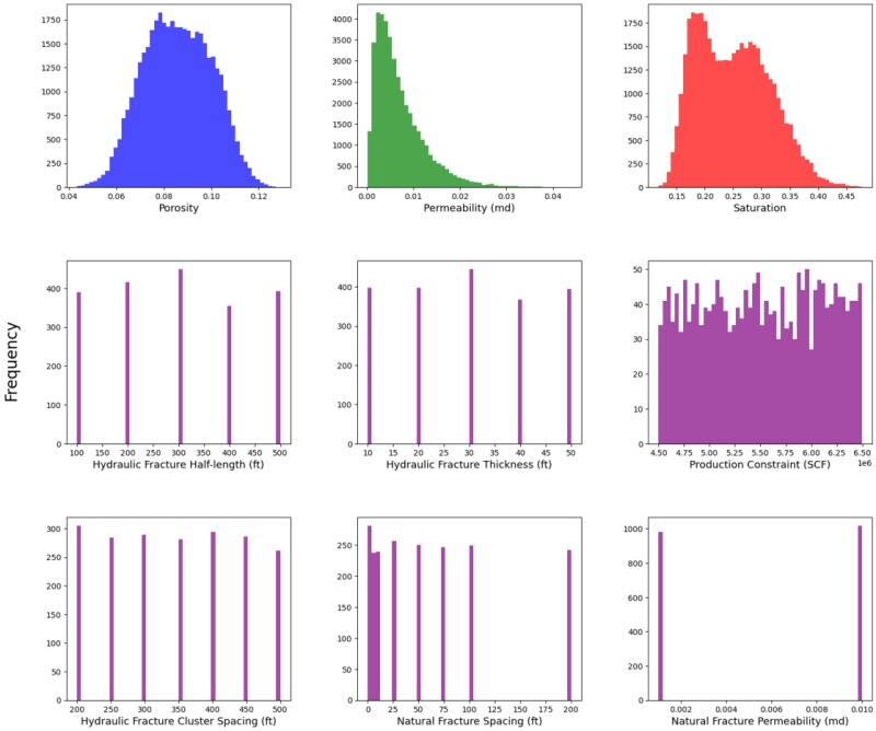
The features in this study were meticulously sampled to cover a broad parameter space, ensuring reliable reservoir models and production profiles. Geological properties such as porosity and water saturation follow normal distributions, while permeability is log-normal, reflecting typical shale characteristics. As shown in Fig. 1, the data set includes nine distinct features per scenario: three represent vertical spatial variability of permeability, porosity, and water saturation across 21 layers, and six are scalar properties for natural and hydraulically induced fracture characteristics.
Completion parameters (i.e., fracture half-length, height, cluster spacing) are discrete, reflecting design constraints. Similarly, natural fracture spacing and permeability are discretely distributed. The production constraint follows a uniform distribution to incorporate varied operating conditions. These distributions provide insight into the data set’s geological and completion characteristics.
Fig. 1—Histogram distributions of geological and completion parameters used in the machine-learning model. The top row shows continuous reservoir properties, with porosity approximately normal, permeability right skewed, and saturation bimodal. The bottom two rows include mostly discrete completion parameters and uniformly sampled variables.
The targets of this study are modeled to reflect realistic production responses of an unconventional shale analogous to the Eagle Ford Shale under different geological and completion conditions. Each production profile is unique, driven by the variations in geological properties (i.e., porosity, permeability, saturation), completion parameters (i.e., fracture spacing, height, and half-length), natural fracture effects, and operational constraints such as production limits. For each realization, the targets consist of monthly gas rate and condensate rate over a 5-year period (61 months). Each of these two targets for a realization contains 61 numerical values representing the production rate decline over the 5-year duration.
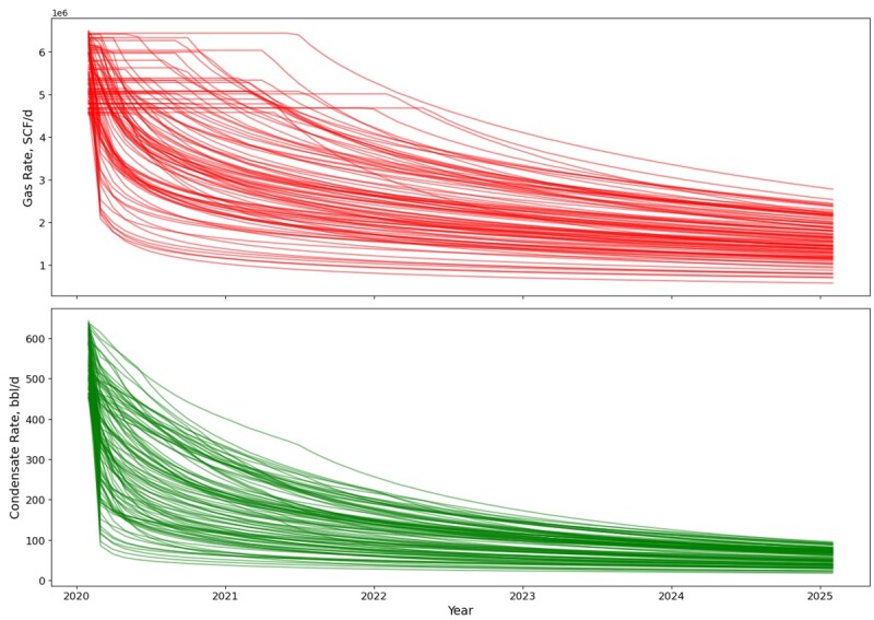
As shown in Fig. 2, these production profiles exhibit significant variability, including sharp initial declines followed by gradual tapering, or short plateaus before slower declines, particularly in gas production. Condensate production rates generally show more gradual declines but also substantial variation. These diverse production patterns are a direct consequence of the variations in the underlying geological and completion parameters and underscore the high heterogeneity and complexity of gas/condensate shale reservoirs, reinforcing the need for robust forecasting models.
Fig. 2—Gas rates (top) and condensate rates (bottom) over a 5-year period for 100 randomly sampled realizations. Each curve represents one realization. The production rates vary significantly because of differences in geological properties and completion designs. Gas rates show a mix of gradual and steep declines, while condensate rates tend to exhibit sharper initial drops followed by slower declines.
The Four Forecasting Models: A Brief Overview The full input feature set is constructed by merging the 63 geological parameters (porosity, permeability, and saturation across 21 layers) with six completion parameters, resulting in a total of 69 features per hydraulically fractured well in the gas/condensate shale formation.
Model 1: Convolutional Neural Network (CNN). The CNN workflow begins with preprocessing: Features are scaled using MinMaxScaler ([0, 1]), and targets are standardized using StandardScaler (mean 0, unit variance) for efficient training. Separate CNN models are developed for gas and condensate rates, both processing the same 69 input features (63 reservoir, six completion). The gas model uses a deeper architecture with three 1D convolutional layers, followed by batch normalization, max-pooling, a 256-neuron dense layer with dropout, and a 61-unit output layer. The condensate model is simpler, with two 1D convolutional layers and similar subsequent layers. Both use ReLU activations in hidden layers and linear output. Training uses the Adam optimizer with a fixed 0.001 learning rate. L2 regularization (lambda = 0.005) and a 0.3 dropout rate are applied to control overfitting. A batch size of 64 is used, and models are trained for up to 100 epochs with EarlyStopping (patience 25) to restore best weights and ReduceLROnPlateau (factor 0.5, patience 15, min_lr 1e−5) for dynamic learning rate adjustment.
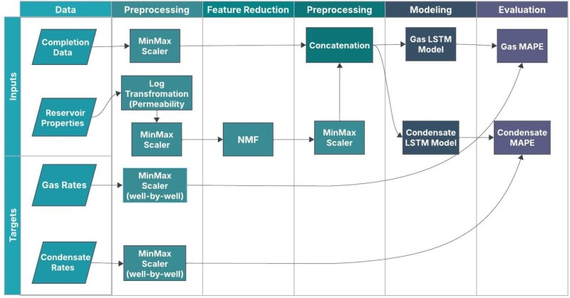
Model 2: Long Short-Term Memory (LSTM) Network With Non-Negative Matrix Factorization (NMF) for Dimensionality Reduction. The LSTM with NMF workflow begins with preprocessing the spatial geological variations. Permeability, which follows a log-normal distribution, is log-transformed for normalization. All input features are then scaled using MinMax scaling. Target production rates are also MinMax-scaled but on a samplewise basis to preserve well-specific trends; the scaling parameters are saved for inverse transformation of predictions to obtain the unscaled targets. To address the high dimensionality of spatial reservoir properties (porosity, permeability, saturation across 21 layers), NMF is applied, decomposing the data into 15 lower-dimensional components while preserving non-negativity and physical meaning to maintain a reconstruction error below 7.5%. Fig. 3 shows the workflow.
LSTM networks are used for time-series regression to capture temporal dependencies in the production data. Separate two-layer LSTM models are trained for gas and condensate rates, using the NMF-transformed reservoir properties combined with completion parameters as input. The architecture was selected based on convergence and manual tuning, using stacked LSTM layers with dropout regularization before a fully connected output layer. Training uses a batch size of 32 and a maximum of 80 epochs, with EarlyStopping (patience 30) to prevent overfitting and restore best weights. Optimal units were 256 and 128 for gas, and 64 and 32 for condensate, with tuned learning rates (0.0006 for gas, 0.02 for condensate) and a dropout rate of 0.1. Architecture was selected based on convergence behavior and manual hyperparameter tuning.
Fig. 3—Production forecasting workflow based on LSTM model with NMF.
Model 3: LSTM Network Without Dimensionality Reduction. This LSTM workflow follows a structure similar to the previous approach but omits dimensionality reduction, such as NMF. The preprocessing phase begins with normalization using MinMaxScaler (0–1 range), while the target production rates are standardized using StandardScaler (mean 0, unit variance) to handle variance effectively. Finally, the input matrix is reshaped to a 3D format (samples, time steps, features) with a timestep of one, as required by LSTM.
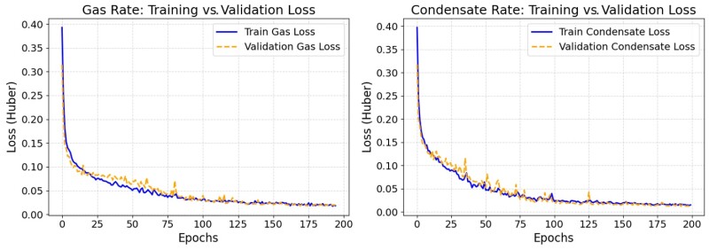
Two separate LSTM models, identical in architecture, are constructed to forecast gas and condensate production rates over 5 years (61 monthly outputs). Each model consists of three stacked LSTM layers, each with 64 hidden units. Dropout (0.1 rate) is applied after each LSTM layer to mitigate overfitting, and LayerNormalization is used after the first two LSTMs for training stability. ReLU activation is used in the first two LSTM layers and Tanh in the final LSTM, followed by a linear Dense layer for the final rate predictions. Training uses the Adam optimizer (0.001 learning rate), a batch size of 64, and the Huber loss function for robustness to outliers. Regularization includes EarlyStopping (patience 20) and ReduceLROnPlateau (patience 15, factor 0.5) to ensure generalization and prevent overfitting. As shown in Fig. 4, the training and validation loss curves exhibit smooth convergence, confirming the effectiveness of the selected configuration.
Fig. 4—Training and validation loss curves for both gas and condensate models. These curves demonstrate that the selected hyperparameters resulted in stable learning, with convergence observed within 200 epochs.
Model 4: Extreme Gradient Boosting (XGBoost). The XGBoost workflow uses two XGBoost regressors to separately forecast gas and condensate production rates. The preprocessing pipeline, determined through trial and error, handles continuous geological data and categorical completion data separately. Continuous data is standardized using StandardScaler, then the geological features are reduced in dimensionality to 10 components using truncated singular value decomposition (TSVD), which captures 95% of the explained variance and is chosen for its suitability for continuous/sparse data and compatibility with XGBoost. Categorical data undergoes no preprocessing to avoid introducing unintended relationships. The transformed continuous data and original categorical columns are then concatenated into a single data frame for model training. The XGBoost model is optimized using GridSearchCV with threefold cross-validation, using negative mean absolute error as the scoring metric for hyperparameter tuning. After generating predictions, a Savitzky-Golay filter is applied to the predicted gas and condensate rate curves. This post-processing step smooths out short-term fluctuations to better reflect the underlying production trend and provide more representative error metrics by avoiding over-penalizing for noise. Fig. 5 shows the XGBoost workflow for the production forecasting.
Fig. 5—XGBoost workflow chart given both geologic and completion parameters, using Standard Scaler and TSVD for preprocessing. A Savitzky-Golay filter is applied to the predicted rates before error evaluation to smooth short-term noise.
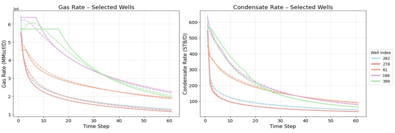
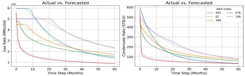
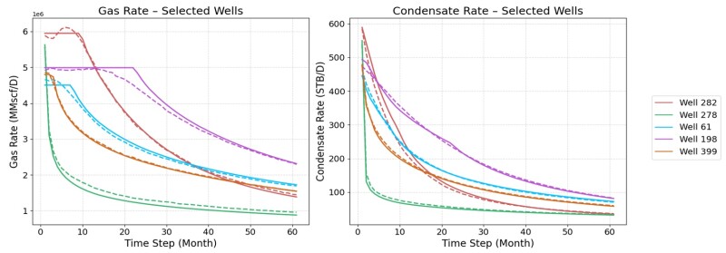
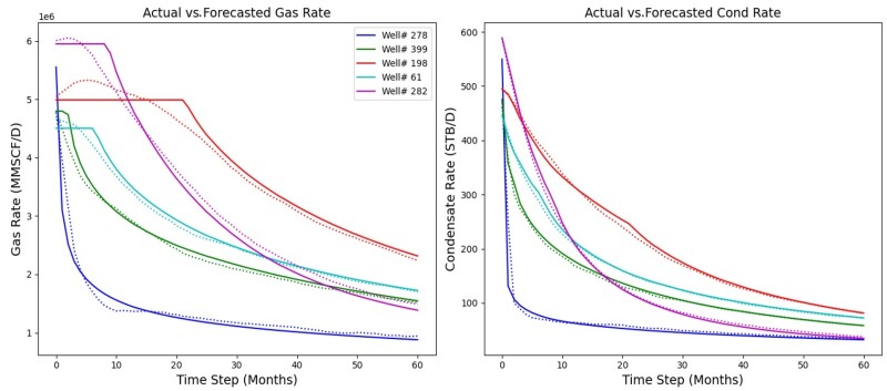
Forecasting Performances of the Four Forecasting Models Figs. 6 through 9 collectively illustrate the forecasting performances of the four predictive workflows, Models 1 to 4, by comparing predicted (in dashed) and actual (in solid) monthly production rates for five randomly selected wells over the 5-year horizon. These plots consistently demonstrate strong alignment between the model’s predictions and the observed data, effectively capturing production trends, rate magnitudes, and decline behavior across a range of well types, including both high- and low-rate producers. While minor discrepancies are observed in some cases, particularly for gas wells exhibiting production plateaus because of constraints, the overall visual correlation between predicted and actual rates confirms the model’s accuracy and robust predictive capability across the majority of test scenarios.
Fig. 6—Actual vs. forecast monthly production rates for CNN-based forecasting.
Fig. 7—Actual vs. forecast monthly production rates for LSTM+NMF-based forecasting.
Fig. 8—Actual vs. forecast monthly production rates for LSTM-based forecasting (without NMF).
Fig. 9—Actual vs. forecast monthly production rates for XGBoost-based forecasting.
Comparative Assessment of the Forecasting Models In this study, we compare three deep-learning workflows —CNN, LSTM networks with and without feature reduction via NMF, and one traditional machine learning based on boosting, XGBoost—on the task to forecast 5 years of monthly gas and condensate production rates for horizontal wells drilled in shale reservoirs. Each of the four forecasting workflows was developed and tuned independently by separate teams using the same data set, allowing for a consistent basis of evaluation.
To provide a holistic comparison, each forecasting model is evaluated not only based on predictive accuracy on the same testing data set but also on model complexity, training time, observed overfitting, and user bias. A summary of these criteria/aspects for the desired comparison is provided in Table 1. Comparing the four data-driven production-forecasting methods across well-defined criteria will furnish a comprehensive and nuanced evaluation of each technique. This systematic comparison will offer clear insights into the trade-offs between crucial aspects such as accuracy, complexity, training efficiency, ease of use, and deployment readiness. Consequently, readers will be empowered to make informed decisions regarding the most suitable method for their specific hydrocarbon production forecasting needs in shale reservoirs, significantly enhancing the practical value and overall effect of this research.
The four techniques are compared based on the following criteria:
Mean and median absolute percentage error (MAPE) in percent—Represents the mean/median of the MAPEs calculated for each well. For example, the median of the MAPE calculated for each well, as shown in the histograms previously mentioned, is used when evaluating the forecasting performances of the four models.
Trainable parameters—Indicates the complexity of each model. Comparing the number of trainable parameters helps in understanding the model’s capacity to learn intricate patterns but also its susceptibility to overfitting and computational demands.
Training epochs—Reflects the number of iterations required for each model to converge during training. Comparing training epochs provides insights into the learning efficiency of each method.
Overfitting observed—Provides qualitative assessment crucial for determining how well each model generalizes to unseen data. A model with significant overfitting, even with good training performance, will likely perform poorly in real-world applications.
Tuning complexity—Assesses the effort and expertise required to optimize the hyperparameters of each model. A lower tuning complexity makes a model more accessible and easier to implement in practice.
Human bias/setup—A qualitative metric that acknowledges the degree to which human decisions (e.g., feature engineering, model architecture selection) might influence the performance of each method. Lower human bias generally leads to more objective and reproducible results.
Ease of use—Reflects the user-friendliness of each method, including aspects such as software availability, documentation, and the learning curve involved in implementation.
Inference time (for 100 samples): Is critical for real-time or near real-time forecasting applications. Comparing inference times helps determine which models are computationally efficient enough for practical deployment.
Robustness—Qualitatively evaluates the stability and reliability of each model’s performance under different conditions or with slightly different data sets. A robust model should maintain consistent predictive power.
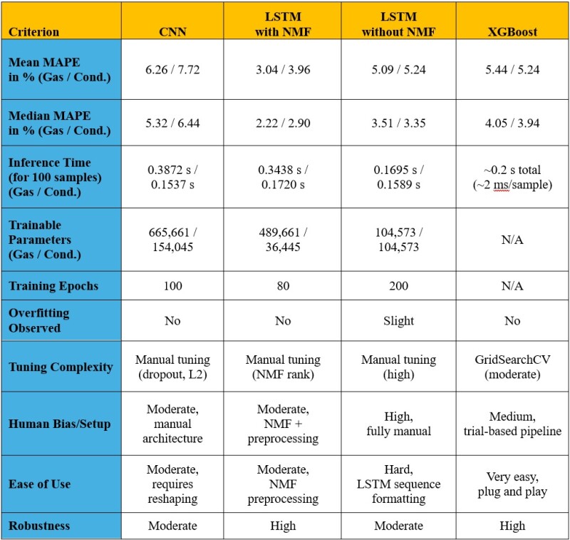
Table 1—Comparative summary of the four production forecasting models’ performance and implementation characteristics. LSTM with NMF achieved the best accuracy, though it required dimensionality reduction and custom preprocessing. CNN and standard LSTM models also performed well but required more manual tuning and input formatting. XGBoost was the most straightforward to use, with competitive accuracy and minimal overfitting observed.
Key Insights From Benchmarking Results his study compares three deep-learning workflows—CNN, LSTM networks with and without feature reduction via NMF, and one traditional machine learning based on boosting, XGBoost—on the task to forecast 5 years of monthly gas and condensate production rates for horizontal wells drilled in shale reservoirs. Each of the four forecasting workflows was developed and tuned independently by separate teams using the same data set, allowing for a consistent basis of evaluation. Each technique was assessed using a diverse set of performance and implementation criteria, offering a well-rounded understanding of their respective strengths and limitations.
Quantitatively, LSTM with NMF demonstrated the highest accuracy, achieving mean MAPEs of 3.04% (gas) and 3.96% (condensate), and median MAPEs of 2.22% (gas) and 2.90% (condensate). This contrasts with CNN (mean MAPE: 6.26%/7.72%; median MAPE: 5.32%/6.44%), LSTM without NMF (mean MAPE: 5.09%/5.24%; median MAPE: 3.51%/3.35%), and XGBoost (mean MAPE: 5.44%/5.24%; Median MAPE: 4.05%/3.94%). LSTM with NMF also exhibited high robustness and no observed overfitting, despite having a moderate number of trainable parameters (489,661 for gas, 36,445 for condensate) and requiring 80 training epochs. This is presented in Table 1.
In contrast, XGBoost, while showing slightly higher MAPE values than LSTM with NMF, demonstrated excellent usability and very fast inference time (approximately 0.2 seconds total for 100 samples, or ~2 ms per sample). It also exhibited no overfitting and moderate tuning complexity (by using GridSearchCV).
CNN and standard LSTM models performed reasonably well in terms of accuracy but required more manual tuning and were more susceptible to overfitting (slight overfitting observed for LSTM without NMF).
The standard LSTM model had fewer trainable parameters (104,573 for both gas and condensate) and a faster inference time (0.1695s/0.1589s for 100 samples) compared with CNN (665,661/154,045 parameters, 0.3872s/0.1537s inference time), making it potentially preferable in some cases despite requiring more training epochs (200) than CNN (100) or LSTM with NMF (80).
Human bias/setup was highest for LSTM without NMF (fully manual) and hard for ease of use (LSTM sequence formatting), while XGBoost was rated medium for human bias/setup (trial-based pipeline) and very easy for ease of use (plug-and-play).
Recommendations Based on the Benchmarking Results The benchmarking results offer crucial insight for real-world applications in the energy industry. While deep learning, particularly the LSTM with NMF approach, can provide superior accuracy for complex production forecasting tasks, its implementation often requires significant data preprocessing, feature-engineering expertise, and computational resources. This makes it highly valuable for scenarios where maximizing predictive precision is paramount and the necessary technical infrastructure and expertise are available.
Conversely, boosting-based methods such as XGBoost, while potentially sacrificing a small degree of accuracy compared with the best-deep learning model, offer a compelling balance of competitive performance, exceptional ease of use, rapid inference time, and lower tuning complexity. This makes XGBoost a highly practical and readily deployable solution for operational environments, rapid screening of scenarios, or situations where interpretability and ease of implementation are key priorities.
The choice between these approaches in practice is not a simple one-size-fits-all decision but rather a strategic trade-off based on the specific needs, available resources, and priorities of the application. This comparative framework empowers practitioners to make informed choices tailored to their forecasting goals and technical constraints, moving beyond simply selecting the most accurate model in isolation. Future efforts should also explore automating preprocessing pipelines and hyperparameter tuning to improve the accessibility and reproducibility of advanced deep-learning methods across diverse production data sets.
Based on these findings, the following recommendations are made:
For highest accuracy in production forecasting, especially when computational resources and expertise are available, LSTM with NMF is recommended. Its performance justifies the added complexity in preprocessing and setup.
For rapid deployment and ease of use, particularly in operational environments with limited machine-learning infrastructure, XGBoost offers the best trade-off between performance and simplicity. It remains robust, scalable, and interpretable with minimal tuning.
For applications where architecture flexibility is desired, CNN and standard LSTM are viable, although they may require more attention to model design, tuning, and data formatting.
Future efforts should consider automating preprocessing pipelines and hyperparameter tuning, particularly for models requiring dimensionality reduction or sequence formatting. This would improve accessibility and reproducibility across diverse production data sets.
This work was supported by the Texas A&M Data Science Institute under the Data Analytics for Petroleum Industry Certificate program, generously funded by ConocoPhillips.